BLOG
Scope 1 & 2 Emission Accounting: Step‑by‑Step Calculations with Real Case Studies | Anaxee
Teaching Calculations: Emission Accounting for Scope 1 & Scope 2
When most sustainability manuals explain greenhouse‑gas (GHG) accounting, they bury you in jargon before getting to the numbers. This article flips the script. We focus squarely on Scope 1 and Scope 2 calculations, walking line‑by‑line through real‑world data sets from four Indian sectors:
- Cement manufacturing (heavy industry)
- Cloud data centre (service + power intensive)
- Bottled beverages plant (FMCG)
- Textile dyeing mill (SME)
For each case study we share raw activity data, pick the right emission factors, crunch the numbers, and reflect on what the results actually mean for management. All examples use FY 2024‑25 data, Indian grid factors, and IPCC Fifth Assessment defaults unless stated otherwise.
Note for beginners – We assume you already know what Scope 1 and Scope 2 are. If not, jump over to our previous primer on GHG boundaries, then hop back here for the math.
1. The Calculation Cheat‑Sheet
Before diving into sector specifics, let’s frame the generic formulas:
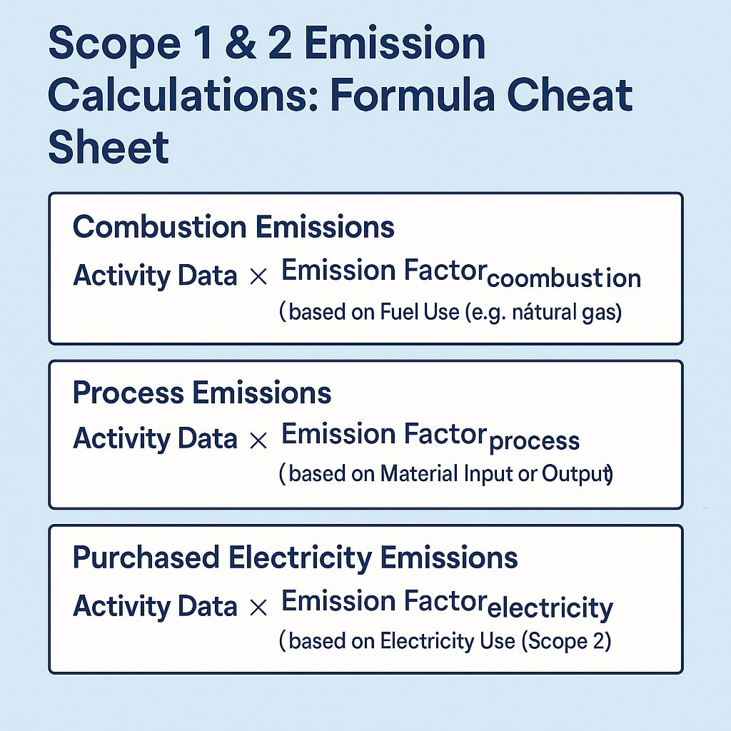
| Source Type | Basic Formula |
| Combustion (liquid fuels) | Activity (litres) × EF (kg CO₂/L) × (1 – Oxidation Factor) |
| Combustion (gaseous fuels) | Activity (scm or kWh) × EF (kg CO₂/unit) |
| Purchased Electricity | Electricity (kWh) × Grid EF (kg CO₂/kWh) |
| Purchased Steam / Chilled Water | Energy (kWh) × Supplier EF (kg CO₂/kWh) |
CH₄ and N₂O for fossil‐fuel combustion are normally added as CO₂‑equivalent using their global‑warming potentials (GWPs). We keep them visible in the cement example so you see the mechanics.
Quick tip – Always store ➞ unit conversions in a corner of your spreadsheet: 1 litre diesel ≈ 0.832 kg; 1 kg natural gas ≈ 1.25 scm (depends on calorific value).
2. Case Study 1 – Cement Plant in Andhra Pradesh
2.1 Activity Data Snapshot (FY 2024‑25)
Activity Unit Quantity Diesel for quarry trucks L 2,500,000 Coal for kiln t 135,000 Grid electricity kWh 78,000,000 On‑site WHR* electricity kWh 12,000,000 *WHR = waste‑heat recovery. Electricity from WHR is counted as zero‑carbon internal generation, not grid purchase.
2.2 Emission Factors Selected
-Diesel: 2.68 kg CO₂/L (IPCC default)
-Coal: 2.42 t CO₂/t (bituminous, India average)
-Grid EF (Southern grid, CEA 2024): 0.72 kg CO₂/kWh
2.3 Scope 1 Calculation – Diesel & Coal
Diesel (mobile)
2,500,000 L × 2.68 kg CO₂/L = 6,700,000 kg CO₂ ≈ 6,700 tCoal (stationary)
135,000 t × 2.42 t CO₂/t = 326,700 tCH₄ and N₂O minor: +0.5 % → 1,633 t CO₂e
Scope 1 subtotal: 334, (6,700 + 326,700 + 1,633) = 335,033 t CO₂e
2.4 Scope 2 Calculation – Purchased Grid Electricity
78,000,000 kWh × 0.72 kg CO₂/kWh = 56,160,000 kg = 56,160 tScope 2 location‑based: 56,160 t CO₂
No market‑based certificates were purchased, so the market‑based number is the same.
2.5 What Management Learned
– Kiln coal dominates (97 % of Scope 1). Even a 5 % thermal‑efficiency improvement would shave 16,000 t CO₂.
– Switching quarry trucks from diesel to electric would cut ~6,700 t—small in percentage terms but big PR value.
– Installing an extra 8 MW WHR turbine could offset another 40 GWh grid power, saving 28,800 t Scope 2.
3. Case Study 2 – Tier‑III Data Centre, Bengaluru
3.1 Activity Data
| Activity | Unit | Quantity |
| Grid electricity (including cooling) | kWh | 42,000,000 |
| Diesel for back‑up generators | L | 420,000 |
3.2 Factors
-Bangalore BESCOM grid EF 2024: 0.79 kg CO₂/kWh
-Diesel EF: 2.68 kg CO₂/L
3.3 Scope 2 First (because it is huge)
42,000,000 × 0.79 = 33,180,000 kg = 33,180 t3.4 Scope 1 Back‑up Diesel
420,000 L × 2.68 = 1,125,600 kg = 1,126 t3.5 Outcome & Actions
-Electricity is 30× bigger than diesel. The company signed a 25‑year solar Open‑Access PPA for 30 GWh/yr.
-Market‑based Scope 2 will drop from 33,180 t to roughly 3,318 t once RECs are matched 90 % of the year.
-Diesel gensets run only 80 hours/year. Replacing with li‑ion battery UPS would also reduce Scope 1 spikes during testing.
4. Case Study 3 – Beverage Bottling Plant, Maharashtra
4.1 Activity Data
| Activity | Unit | Quantity |
| LPG for boilers | t | 1,200 |
| Purchased steam from neighbour CHP | t steam | 85,000 |
| Grid electricity | kWh | 18,500,000 |
4.2 Factors
-LPG EF: 3.00 t CO₂/t LPG (WTT included)
-Steam supplier EF (metered): 0.25 t CO₂/t steam
-Western grid EF 2024: 0.78 kg CO₂/kWh
4.3 Calculations
LPG (Scope 1)
1,200 t × 3.00 = 3,600 tPurchased Steam (Scope 2 – heat)
85,000 t × 0.25 = 21,250 tGrid Electricity (Scope 2 – power)
18,500,000 kWh × 0.78 kg/kWh = 14,430 t4.4 Result Summary
| Scope | t CO₂e |
| 1 | 3,600 |
| 2 (power) | 14,430 |
| 2 (steam) | 21,250 |
| Total Scope 2 | 35,680 |
Purchased steam is the surprise hotspot. Management is negotiating to co‑locate a biomass boiler that would slash Scope 2 by 70 %.
5. Case Study 4 – Textile Dyeing Mill, Tamil Nadu
5.1 Activity Data
| Activity | Unit | Quantity |
| Furnace oil | L | 600,000 |
| Grid electricity | kWh | 9,600,000 |
5.2 Factors
-Furnace oil EF: 3.12 kg CO₂/L
-TN grid EF 2024: 0.69 kg CO₂/kWh
5.3 Calculations
Scope 1: Furnace Oil
600,000 L × 3.12 kg/L = 1,872,000 kg = 1,872 tCH₄, N₂O negligible (<1 %).
Scope 2: Grid Power
9,600,000 kWh × 0.69 kg/kWh = 6,624,000 kg = 6,624 t5.4 Insights
-Although a small SME, electricity is 3.5× larger than oil. Rooftop solar (2.5 MWp) can offset ~4,000 t Scope 2.
-Switching from furnace oil to LPG reduces both CO₂ and local particulates—useful for compliance with TN PCB.
6. Common Pitfalls When Teaching Scope 1 & 2 Accounting
- Mixing units – Litres vs kilograms. Embed conversion factors in your template.
- Wrong grid factor vintage – Always cite the reporting year (CEA publishes annually). Investors notice.
- Double counting captive renewables – If you own a rooftop solar array, subtract its kWh from grid purchase before applying the grid EF.
- Ignoring oxidation factors – Most liquid fuels are 100 %, but coal can be 98 %. Check IPCC tables.
- Rounding too early – Keep at least three significant figures through the math; round only in the final report.
7. Bringing It All Together – A Template Walk‑Through
Below is a simplified template header. Copy into Excel/Sheets and replicate rows per source.
| Site | Year | Source | Fuel/Utility | Unit | Quantity | EF | EF Source | Scope | t CO₂ | Notes |
Populate Source with diesel genset, grid power, LPG boiler, etc. The formula for t CO₂ is simply Quantity*EF/1000 if EF is in kg CO₂/unit.
Pro hint – Colour‑code Scope 1 rows red and Scope 2 blue; the pattern helps non‑experts spot which bars must shrink.
8. FAQ – Calculation Edition
Q: Which emission‑factor database is “best” for India?
A: The Central Electricity Authority’s regional grid mix is mandatory for BRSR. For fuels, default to IPCC but cross‑check with India GHG Program if available.
Q: Do I count solar power I export?
A: Exported electricity is deducted from your grid import before calculating Scope 2. The residual export may be reported as avoided emissions in a footnote, but not subtracted from Scope 1.
Q: How to show location‑ vs market‑based numbers?
A: Two separate rows in your disclosure. Make it clear which one ties to targets and which one goes to CDP.
9. Key Takeaways for Trainers & Learners
-Always start with high‑quality activity data. Fancy EFs can’t rescue garbage inputs.
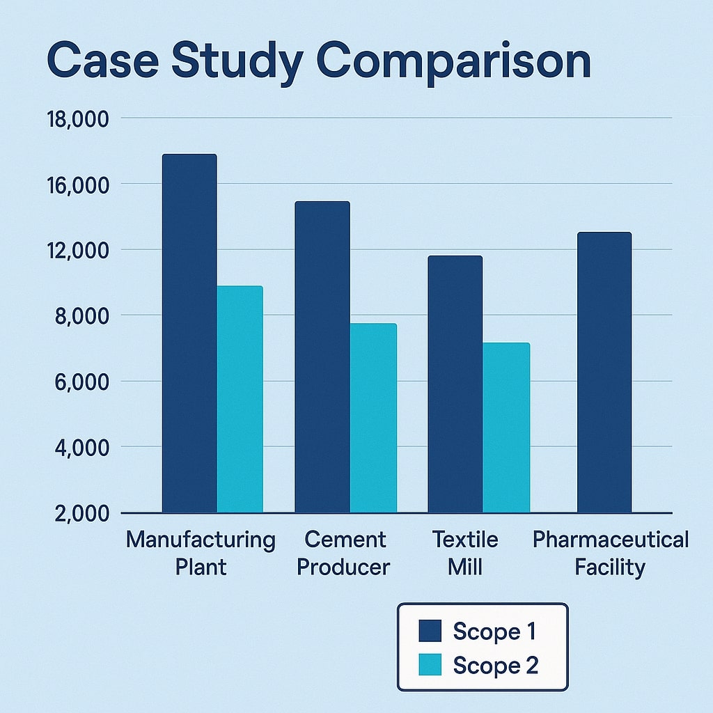
-Visualise the result (bar chart Scope 1 vs Scope 2) so management intuitively grasps priorities.
-Use sector‑relevant stories—cement, data centres, FMCG—because numbers stick when anchored in reality.
-Iterate annually; the more often teams run the calculations, the faster they spot anomalies and savings.
10. Conclusion
Scope 1 and Scope 2 may be “only” the first two slices of the carbon pie, but they often dictate over 90 % of what a company can directly control in the next five years. By mastering the calculations shown above- diesel, coal, LPG, grid electricity, and purchased steam—you arm yourself with a decision‑making compass.
From slashing diesel in quarry trucks to inking renewable‑energy PPAs, the path to lower emissions starts with a spreadsheet and a clear line of sight to each tonne of CO₂. Now roll up your sleeves, grab last year’s utility bills, and teach your team the math.
About Anaxee:
Anaxee is India’s Reach Engine! we are building India’s largest last-mile outreach network of 100,000 Digital Runners (shared feet-on-street, tech-enabled) to help Businesses and Social Organizations scale to rural and semi-urban India, We operate in 26 states, 540+ districts, and 11,000+ pin codes in India.
We Help in last-mile execution of projects for (1) Corporates, (2) Agri-focused companies, (3) Climate, and (4) Social organizations. Using technology and people on-the-ground (our Digital Runners), we help in scale and execute projects across 100s of cities and bring 100% transparency in groundwork. We also work in the Tech for Climate domain, providing technology for the execution and monitoring of Nature-Based (NbS) and Community projects. Our technology & processes bring transparency and integrity into carbon projects across various methodologies (Agroforestry, Regen Agriculture, Solar devices, Improved Cookstoves, Water filters, LED lamps, etc.) worldwide.
For More info or query, Connect with sales@anaxee-wp-aug25-wordpress.dock.anaxee.com